Monte Carlo Simulation
A single backtest gives you one trade sequence — the one that happened to occur historically. But the order of those trades wasn't preordained: the same strategy with the same trades arranged in a different sequence could have produced a 30% drawdown instead of a 12% one. Monte Carlo simulation stress-tests your strategy by running thousands of randomized variations of your backtest results, so you see the full distribution of possible outcomes rather than the single number a backtest produces.
VolatiCloud supports up to 50,000 iterations per simulation, three randomization methods (Trade Shuffle, Bootstrap, Parametric), full equity curve confidence bands, and a configurable Risk of Ruin threshold.
What Monte Carlo Simulation Does
Imagine you have a backtest that produced 200 trades. Those trades happened in a specific order dictated by the market. But what if the market had arranged those same opportunities differently? What if some trades happened more frequently than others?
Monte Carlo simulation answers these "what if" questions by:
- Taking your historical trades from a completed backtest
- Randomizing them thousands of times (shuffling order, resampling, or generating synthetic trades)
- Recalculating performance metrics for each randomized version
- Showing you the distribution of possible outcomes rather than a single number
The result is a confidence range: instead of "my strategy returned 45%," you learn "my strategy returns between 20% and 65% in 90% of scenarios."
Why Use Monte Carlo on Crypto Backtests?
A single backtest result can be misleading. Monte Carlo simulation helps you understand:
| Single Backtest | Monte Carlo |
|---|---|
| "I made 45% profit" | "I make between 20% and 65% in 90% of scenarios" |
| "Max drawdown was 15%" | "There's a 10% chance drawdown exceeds 30%" |
| "Sharpe ratio is 1.8" | "Sharpe ratio ranges from 0.9 to 2.4" |
Key Benefits
- Detect overfitting — if results vary wildly across permutations, your strategy may be overfit to the specific trade sequence (see the avoiding overfitting guide)
- Quantify risk — understand the probability of large drawdowns or account ruin
- Build deployment confidence — a strategy with tight confidence bands is more robust than one with wide bands
- Compare strategies — two strategies with similar single-backtest returns may have very different risk profiles under Monte Carlo analysis
Monte Carlo uses your historical trades as the basis for randomization. It cannot predict how your strategy will perform in fundamentally different market conditions (e.g., a black swan event). It tells you about the range of outcomes given the types of trades your strategy has historically produced.
How Monte Carlo Simulation Works
VolatiCloud supports three simulation methods, each designed for different analytical questions.
Trade Shuffle
What it does: randomly reorders your trades and recalculates the equity curve for each permutation.
What it answers: "How much does the sequence of trades matter to my final result?"
Example: your backtest had 3 winning trades followed by 3 losing trades. Trade shuffle might produce a sequence like: win, lose, win, lose, win, lose. The total profit is the same, but the equity curve path and maximum drawdown are different.
Best for: understanding path dependency and drawdown risk. This is the recommended default method.
Bootstrap
What it does: samples trades with replacement from your trade history. In each iteration, some trades appear multiple times while others are omitted entirely.
What it answers: "What if certain types of trades happened more or less frequently?"
Example: if your strategy has 100 trades, each bootstrap iteration picks 100 trades randomly from that pool. A highly profitable trade might appear 3 times in one iteration and 0 times in another, changing the overall result.
Best for: understanding sensitivity to individual trade outcomes. If a few large winners drive your performance, bootstrap will reveal this dependency.
Parametric
What it does: fits a normal (bell curve) distribution to your trade returns, then generates entirely synthetic trades drawn from that distribution.
What it answers: "What does my performance look like under idealized statistical assumptions?"
Example: if your average trade return is 1.2% with a standard deviation of 3.5%, the parametric method generates thousands of synthetic trades from a N(1.2%, 3.5%) distribution.
Best for: generating smooth distributions and testing performance under theoretical assumptions. Useful when your trade count is small (< 30 trades).
Which method should I use? Start with Trade Shuffle — it makes the fewest assumptions about your data and directly answers the most common question: "How dependent is my result on trade ordering?" Use Bootstrap when you want to understand sensitivity to individual trades, and Parametric when you have very few trades.
Method Comparison
| Feature | Trade Shuffle | Bootstrap | Parametric |
|---|---|---|---|
| Trade count preserved | Yes | Yes | Configurable |
| Trade values preserved | Yes | Yes (resampled) | No (synthetic) |
| Tests order dependency | Yes | Partially | No |
| Tests frequency sensitivity | No | Yes | No |
| Works with few trades (< 30) | Limited insight | Limited insight | Good |
| Assumptions | None | Independence | Normal distribution |
Understanding Monte Carlo Results
After a simulation completes, you see several result panels.
Equity Curve Bands
The equity curve chart shows five colored bands representing different percentile outcomes:
| Band | Color | Meaning |
|---|---|---|
| p95 | Light green | Best-case scenario (only 5% of simulations did better) |
| p75 | Green | Above-average outcome |
| p50 | Blue | Median outcome — the "typical" result |
| p25 | Orange | Below-average outcome |
| p5 | Red | Worst-case scenario (only 5% of simulations did worse) |
How to interpret: a narrow band (p5 and p95 are close together) means your strategy performs consistently regardless of trade ordering. A wide band suggests high sensitivity to the specific sequence of trades.
Final Balance Distribution
A histogram showing the distribution of final account balances across all iterations.
- Mean — average final balance
- Median (p50) — the "typical" final balance (more robust than mean if outliers exist)
- Standard deviation — how spread out the results are
If the mean is significantly higher than the median, a few extreme winning scenarios are pulling the average up. The median is a more reliable expectation.
Risk of Ruin
Shows the probability of your account balance dropping below a configured threshold during any simulation run. You configure a single riskOfRuinThreshold percentage (default: 50%), and the engine calculates the fraction of simulations where the balance fell below that level.
How it works:
- The ruin line is calculated as
initialCapital * (1 - riskOfRuinThreshold / 100). For example, with $10,000 initial capital and a 50% threshold, the ruin line is $5,000. - For each simulation iteration, if the balance dropped below the ruin line at any point, that iteration counts as "ruin."
- Risk of Ruin = number of ruin iterations ÷ total iterations. The result is a single probability between 0% and 100%.
Example: with a 50% threshold and 1,000 iterations, if 3 iterations saw the balance dip below 50% of initial capital, Risk of Ruin = 0.3%.
Target: risk of ruin should be near zero for a robust strategy. If it exceeds a few percent, consider reducing position sizes or adding stop-loss rules. You can adjust the riskOfRuinThreshold to test different loss levels (e.g., set it to 25 to check the probability of losing 25% of capital).
Drawdown Distribution
Shows the distribution of maximum drawdown values across all iterations. Similar to final balance, but focuses on the worst peak-to-trough decline in each iteration.
Sharpe and Sortino Distributions
Histograms of risk-adjusted return metrics across iterations:
- Sharpe ratio — return divided by total volatility. Target: > 1.0 in the median (p50)
- Sortino ratio — return divided by downside volatility only. Target: > 1.5 in the median
A Sharpe ratio that stays above 1.0 even at p5 indicates a consistently risk-efficient strategy.
Advanced Monte Carlo Configuration
| Parameter | Default | Range | Description |
|---|---|---|---|
| Iterations | 1,000 | 10–50,000 | Number of Monte Carlo iterations. More iterations = smoother distributions but longer runtime |
| Method | trade_shuffle | trade_shuffle, bootstrap, parametric | Simulation method (see above) |
| Initial Capital | From backtest | Any positive number | Starting account balance for equity curve calculation |
| Confidence Levels | 5, 25, 50, 75, 95 | Any percentiles (0–100) | Which percentile bands to compute |
| Seed | Random | Any integer (as string) | Set a fixed seed for reproducible results. Accepts 64-bit integers (e.g., nanosecond timestamps) |
| Include Fees | true | Boolean | Whether to include trading fees in the simulation. When enabled, fees are deducted from PnL during equity curve calculation |
| Fee Rate | (not set) | 0–1.0 (optional) | Custom fee rate to use instead of the backtest's original fee amounts. Expressed as a decimal (e.g., 0.001 = 0.1%). When set, overrides the per-trade fees from the backtest |
| Risk-Free Rate | 0 | 0 to < 1.0 | Annualized risk-free rate used for Sharpe and Sortino ratio calculations. Expressed as a decimal (e.g., 0.05 = 5%) |
| Risk of Ruin Threshold | 50 | > 0–100 | The percentage loss threshold for Risk of Ruin calculation. A value of 50 means "probability of losing 50% of initial capital" |
Iteration count guidance:
- 1,000 — quick exploration, good for initial checks (< 10 seconds)
- 5,000 — solid analysis, smooth distributions (< 30 seconds)
- 10,000 — publication-quality results (< 60 seconds)
- 50,000 — maximum precision, Enterprise only (1–3 minutes)
Best Practices for Monte Carlo Analysis
Interpreting Results
-
Look at p5, not the mean. The 5th percentile tells you what happens in bad scenarios. If p5 is still profitable, your strategy is robust.
-
Compare methods. Run both Trade Shuffle and Bootstrap. If results differ significantly, your strategy is sensitive to both trade ordering and individual trade outcomes.
-
Check risk of ruin first. Before celebrating returns, verify that the probability of a 30%+ drawdown is acceptably low for your risk tolerance.
-
Use seeds for comparison. When comparing two strategy versions, use the same seed so differences in results reflect strategy changes, not randomization differences.
-
More trades = better analysis. Monte Carlo is most informative with 50+ trades. With fewer than 30, consider using the Parametric method or running longer backtests.
Common Mistakes
Don't cherry-pick methods. If Trade Shuffle shows poor results but Parametric looks good, the strategy likely has order-dependency issues. The conservative (worst) result is the one to trust.
- Ignoring wide confidence bands — if p5 and p95 are far apart, the strategy is inconsistent. Tightening the band (e.g., adjusting position sizing or adding filters) is more important than chasing higher returns.
- Too few iterations — with only 100 iterations, percentile estimates are noisy. Use at least 1,000 for meaningful results.
- Confusing Monte Carlo with forward testing — Monte Carlo reshuffles historical trades. It does not simulate future market conditions. Always combine Monte Carlo analysis with paper trading before deploying live, and consider walk-forward optimization for a complementary check on parameter stability across time.
Plan Requirements
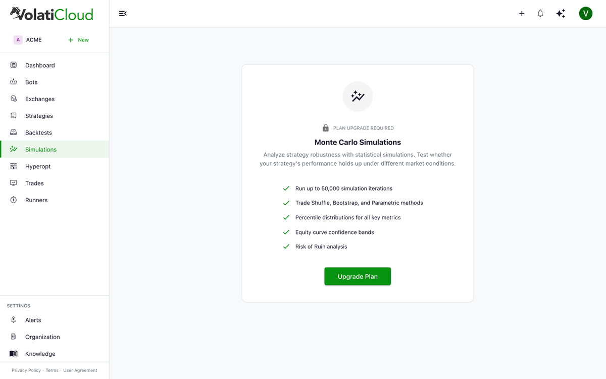
Monte Carlo simulation is available on Pro and Enterprise plans.
| Pro | Enterprise | |
|---|---|---|
| Access | Full | Full |
| Max concurrent simulations | 3 | 10 |
| Max iterations per simulation | 50,000 | 50,000 |
Starter plan users can upgrade to Pro to access Monte Carlo simulation. See Plans & Pricing for details.
Quick Start: Run Your First Monte Carlo Simulation
Step 1: Complete a backtest
Monte Carlo simulation requires trade data from a completed backtest. If you haven't run one yet, see Running a Backtest.
Step 2: Open Simulation
From your completed backtest results page, click Run Monte Carlo Simulation. Alternatively, navigate to your strategy page and select the Simulations tab.
Step 3: Configure
- Select a backtest — choose which backtest's trades to analyze
- Choose a method — start with Trade Shuffle (recommended)
- Set iterations — 1,000 for a quick check, 5,000+ for thorough analysis
- Initial capital — defaults to your backtest's starting capital
Step 4: Run
Click Run Simulation. You'll see real-time progress updates as iterations complete. A typical 1,000-iteration simulation finishes in under 10 seconds.
Step 5: Interpret Results
- Check Risk of Ruin — is the probability of a 30% drawdown acceptable?
- Review Equity Curve Bands — are the bands narrow (consistent) or wide (volatile)?
- Compare Final Balance Distribution — is the median (p50) close to your single backtest result?
- Examine Sharpe/Sortino distributions — does the median stay above 1.0/1.5?
If results look good across all metrics, your strategy has statistical evidence of robustness. If the bands are wide or risk of ruin is high, consider adjusting your strategy parameters before deploying live.
Next Steps
- Running a Backtest — generate trade data for simulation
- Analyzing Backtest Results — understand your base metrics
- Hyperparameter Optimization — tune parameters before stress-testing
- Walk-Forward Optimization — complementary check on parameter stability across time
- Plans & Pricing — upgrade to Pro for Monte Carlo access