Crypto Backtesting Deep Dive: Sharpe, Drawdown, Profit Factor

A strategy that returns 84% over two years on paper means nothing if you can't say what range of outcomes you might actually experience when you run it live. The single number is a starting point — what comes next is rigorous backtesting against years of OHLCV data, multi-pair stress tests, and risk-adjusted metrics like Sharpe and Sortino. VolatiCloud runs that pipeline on Freqtrade's production-tested engine, returns results in seconds to minutes, and surfaces every metric you need to decide whether the strategy survives contact with reality.
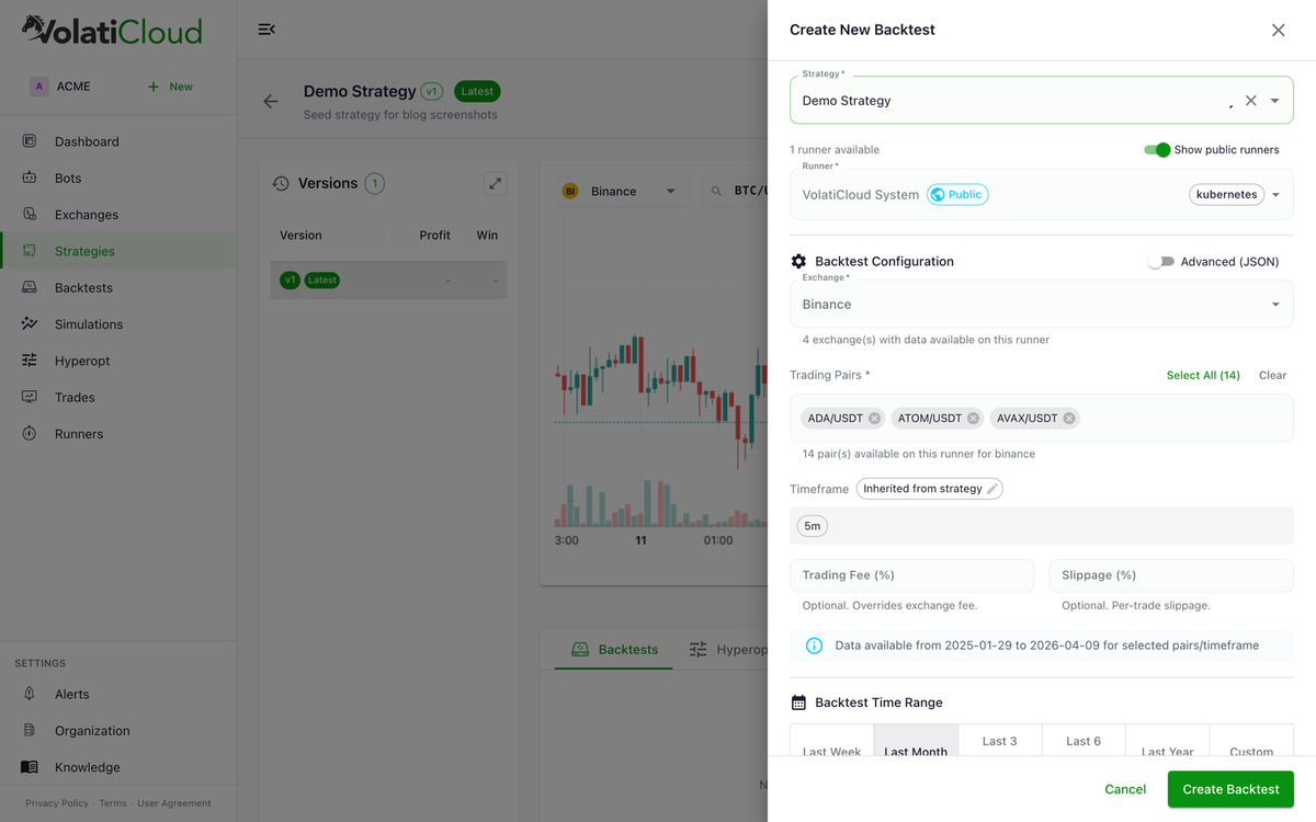
Why Backtest Crypto Strategies Before Going Live
A backtest simulates how your strategy would have performed on historical price data. The questions it answers are the same ones you'd ask before deploying real capital:
- Would this strategy have been profitable across the last 2–3 years?
- What was the worst drawdown you would have lived through?
- How many trades per week or month does it generate (is the sample large enough to trust)?
- Does it perform in bull markets, bear markets, or both?
- Does it work across pairs, or only on the one you tuned it on?
Without backtesting, you're trading on intuition alone. Intuition is fine for hypothesis generation; it's not fine for capital allocation.
Inside the VolatiCloud Backtesting Engine
VolatiCloud uses Freqtrade's backtesting engine — the same engine thousands of algorithmic traders run locally, exposed through a managed UI with the OHLCV data already pre-loaded:
- Candle-by-candle simulation with full OHLCV resolution
- Fee modeling — exchange-specific maker/taker fees applied to every fill
- Slippage approximation — realistic fill price modeling, not "filled at the close"
- 15 timeframes — 1-minute through monthly candles
- 14 supported exchanges — historical data from Binance, Bybit, Kraken, OKX, and more (see supported exchanges)
- Multi-pair backtests — run dozens of pairs in a single backtest, with per-pair breakdowns
For details on data availability per exchange, see the historical data availability post.
Key Backtest Metrics: What to Look At First
A profitable total-return number is necessary but not sufficient. The metrics below are the ones that actually predict whether a strategy survives live trading.
Sharpe Ratio: Risk-Adjusted Return
The Sharpe ratio measures return relative to total volatility. A strategy returning 20% per year with violent equity-curve swings is less attractive than one returning 15% on a smooth path.
Sharpe = (Annual Return − Risk-Free Rate) / Annual Volatility
Target: > 1.0 (excellent: > 2.0). Below 1.0 generally means returns aren't compensating for the volatility you're carrying.
Sortino Ratio: Punishing Only Downside
Sortino is the risk-aware version of Sharpe that ignores upside volatility. Big winning days don't count against you — only the losses do.
Target: > 1.5. Particularly useful for trend-following strategies, which by design have asymmetric upside.
Profit Factor: Gross Wins vs Gross Losses
Profit Factor = Gross Profit / Gross Loss
A profit factor of 1.5 means you made $1.50 on winning trades for every $1.00 lost on losing trades. Target: > 1.5 (excellent: > 2.0). Anything below 1.0 is a losing strategy in expectation.
Max Drawdown: The Number That Predicts Whether You'll Stop the Bot
The worst peak-to-trough decline in equity. A 30% max drawdown means the bot was, at its worst, down 30% from its previous high.
The honest test: Can you psychologically and financially handle the worst-case drawdown without disabling the bot? If a 20% drawdown would make you panic-stop a profitable strategy, you need either tighter risk controls or smaller position sizes — not a different strategy.
Target: < 20% for most retail strategies. Funds may target < 10%.
Win Rate vs Expectancy: Why Win Rate Alone Lies
A 70% win rate sounds great until you realize the average loss is 4× the average win. The combined metric you want is expectancy:
Expectancy = (Win Rate × Average Win) − (Loss Rate × Average Loss)
A strategy with a 40% win rate is highly profitable if winners are 3× the size of losers. A 70% win rate is worthless if losers are 5× the size of winners.
Running a Backtest Step by Step
- Open your strategy in the console
- Click Run Backtest
- Configure:
- Exchange — source of historical OHLCV
- Pairs — single pair or multi-pair set (10+ pairs is reasonable for diversification)
- Date range — at least 12 months for confidence; 2–3 years for high confidence; include both trending and ranging regimes
- Stake amount — capital allocated per trade
- Timeframe — must match your strategy's defined timeframe
- Click Run
Results land in seconds for short ranges, a few minutes for multi-year multi-pair runs. The full step-by-step is in the running backtests doc.
Reading Results: A Worked Example
A representative output for a momentum strategy:
Period: Jan 2024 – Jan 2026 (2 years)
Pairs: BTC/USDT, ETH/USDT, BNB/USDT

Total Profit:        +84.2%
Win Rate:            61%
Profit Factor:       1.73
Max Drawdown:        14.3%
Sharpe Ratio:        1.62
Sortino Ratio:       2.11
Total Trades:        342
Avg Trade Duration:  8.2 hours
Reading this:
- Profitable across both bull and bear regimes (Jan 2024–Jan 2026 covered both)
- Solid win rate (61%) and profit factor (1.73) — the edge is genuine
- Drawdown (14.3%) is acceptable for most retail traders
- Sharpe of 1.62 is strong — risk-adjusted return, not just gross
- 342 trades is well above the 30-trade statistical-significance floor
This is a strategy worth promoting to dry-run mode for live-data validation before committing real capital. The analyzing results doc walks through every metric in the output panel.
Common Backtesting Mistakes
Overfitting to a Specific Date Range
If you tuned your strategy until it looked great on Jan 2024–Jan 2025, it may not generalize to Feb 2025 onward. Always validate on out-of-sample data — a date range you didn't see while building. The avoiding overfitting post covers walk-forward validation, holdout periods, and the specific tells that signal an overfit strategy.
Too Few Trades
Below 30 trades, your win rate, profit factor, and Sharpe are all dominated by noise. Extend the date range, add pairs, or shorten the timeframe to get statistical significance.
Ignoring Market Regimes
A strategy that thrives in trending markets may collapse in chop. Run separate backtests on a clearly trending period and a clearly ranging period — and look at the per-regime metrics, not just the aggregate.
Unrealistic Stop-Losses
A 1–2% stop-loss looks great in backtests because the engine fills cleanly at the stop price. In live trading, a tight stop in a volatile market triggers on noise — and you exit before the move. Calibrate stops to actual market volatility; the ATR stop-loss strategy guide explains how.
From Backtest to Live: The Promotion Path
A backtest is the first gate, not the only gate.
- Backtest — establishes the theoretical edge
- Dry run (paper trading) — validates real-time execution; broker-side latency, partial fills, and stale data show up here
- Live with a minimum stake — confirms the strategy survives contact with real fees and slippage
- Scale up position size as confidence grows
Never skip the dry run. Live execution has different characteristics than candle-replay backtesting — market impact, API latency, and live order book dynamics all affect results. The paper trading to live guide covers the full promotion checklist.
Stress-Testing Beyond the Single Backtest
A single backtest shows you one path through history. But the order your trades happened to occur in is one of thousands of possible sequences. Monte Carlo simulation randomizes the trade order and shows you the full distribution of outcomes — your equity curve at the 5th, 50th, and 95th percentile of plausible histories. The Monte Carlo post walks through how to read p5/p95 bands and risk-of-ruin figures.
For parameter selection, hyperparameter optimization explores the parameter space far more efficiently than manual trial and error — with the same overfitting safeguards.
Open a strategy in the console, click Run Backtest, pick at least 12 months of data, and review the metrics covered above. Once the result holds up across an in-sample and a holdout period, promote it to dry run.
Related guides
- Backtesting Overview — Concepts, metrics, and how the Freqtrade engine runs simulations.
- Running a Backtest — Step-by-step walkthrough for launching your first backtest.
- Avoiding Overfitting in Backtests — Practical techniques to build strategies that generalize.
- Monte Carlo Simulation — Stress-test your strategy with randomized trade sequences.